In this section, the overall architecture of the proposed HREA system shown in Fig. 1 (Fig. 1a shows the overall workflow of the system) is established by the following steps: (a) a rehabilitation exercise and assessment system (consisting of software and wearable sensors) is developed and used to collect rehabilitation data; (b) a basic model is trained on a public dataset and uploaded to the cloud; and (c) a pretrained model stored in the cloud can be used as an initial model for new local tasks. This methodology can significantly reduce training time while concurrently enhancing the model’s generalization capabilities and adaptability.

Overall framework of the HREA system: (a). overall workflow of the HREA system; (b). standard placement of sensors on a physician; (c). user trains following standard action guidance.
The whole system consists of three parts: the patient client, the physician client and the web server. Patients wear the wearable sensors first and finish the rehabilitation plans made by physicians. During the exercise period, the sensors record the movement data, transmit it to the computer via the ZigBee protocol and finally upload it from the computer to the web server through the Internet. The sensor is powered by a lithium-ion battery whose capacity is 400 mAh. When the battery is fully charged, the sensor can continuously operate for 10 h. Physicians can view the patients’ training records and Fugl-Meyer assessment via the website and adjust the individualized movement prescriptions according to the assessment. The work primarily focuses on the design of the “patient client” component within a rehabilitation system.
Each wearable sensor consists of an accelerometer, a gyroscope and a magnetometer, which can capture 3D posture data of the human body. The microprocessor unit sensor chip is a mpu9150 with an accelerometer resolution of ± 16 g, a magnetometer resolution of 4800µT and an angular resolution of 2000 degrees per second. These settings enable the measurement of inclination changes less than 0.1 degrees, which is sensitive enough to capture movement features. The sampling frequency of all sensors is set to 30 Hz. We use the Kalman filter to estimate the attitude angle in the sensor and transmit it to the computer, the estimation process is as follows.
Prediction steps:
$$\beginarrayc\widehatX_k=F\cdot \widehatX_k,\, state\; estimation\endarray$$
(1)
$$\beginarraycP_k-1=F\cdot P_k-1\cdot F^T+Q,\, covariance\; matrix\; estimation\endarray$$
(2)
Update step:
$$\beginarraycK_k=P_k-1\cdot H^T\cdot (H\cdot P_k\cdot H^T+R)^-1,\, Kalman\; gain\endarray$$
(3)
$$\beginarrayc\widehatX_k=\widehatX_k-1+K_k\cdot (Z_k-H\cdot \widehatX_k-1),\, state\; update\endarray$$
(4)
$$\beginarraycP_k=(I-K_k\cdot H)\cdot P_k-1,\, covariance\; matrix\; update\endarray$$
(5)
State vector: \(X=[\phi , \theta , \psi ,\dot\phi , \dot\theta , \dot\psi ]^T\), ϕ, θ, ψ are the roll, pitch and yaw angles, respectively, and \(\dot\upphi \), \(\dot\uptheta \), \(\dot\uppsi \) are the corresponding angular velocities.
Measurement vector: \(Z=[a_x,a_y, a_z,\omega _x,\omega _y,\omega _z,b_x,b_y,b_z]^T\), \(a_x,a_y, a_z\) are accelerometer readings, \(\omega _x,\omega _y,\omega _z\) are the gyroscope readings, and \(b_x,b_y,b_z\) are the gyroscope readings.
F is the state transfer matrix, H is the measurement matrix, P is the covariance matrix and I is the initial state.
In this paper, we employ two wearable sensors to conduct the experiment. The hardware cost of the HREA system is less than $50, which can be afforded by patients. The locations of the sensors are shown in Fig. 1b. The sensors were placed in the geometric central area of the upper limbs and elastic bandages were used to keep the sensor firmly attached to the tissue. Sensor 2 (#S2) was placed at a position at least 10 cm away from both the elbow and shoulder, while sensor 1 (#S1) was placed on the forearm within 5 cm of the wrist. We record the attitude angle data of the patient’s rehabilitation training and use it as input for the model.
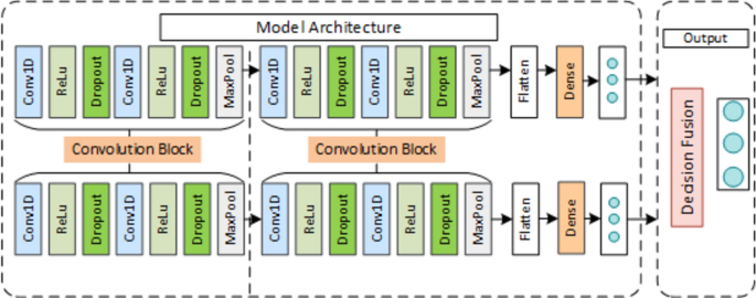
A multichannel 1D-CNN model is proposed in this section. As shown in Fig. 2, the assessment model consists of two submodels(1D-CNN) and a decision fusion module. We use the submodel to assess each sensor channel separately and then feed the output predicted values into the decision module as inputs to obtain the final score.

Diagram of the multichannel 1D-CNN architecture for rehabilitation exercise assessment.
Preprocessing
To reduce the influence of signal difference, all data obtained from the wearable sensor are normalized to the range of [− 1, 1] using the standard min–max normalization as follows:
$$\beginarraycx_i=\fracx_i-x_minx_max-x_min\endarray$$
(6)
where \(x_i\) represents the motion posture value of the i-th sampling point of the action recording \(x\). It is worth noting that in this paper, unlike in general normalization, \(x_max\) and \(x_min\) are not the calculated results of each data channel. Ideally, the normalization parameters correspond to the sensor measurement range of each action. In practice, depending on the type of action and the different sensor data channels, these parameters are set to different fixed empirical values.
Figure 3 shows the signal of the sensor channel corresponding to a complete rehabilitation action captured with the HREA system. Each sensor channel contained 3 channels of attitude angle, as shown in Fig. 7a. The raw signal was normalized before being input into the model using the default sensor range as the normalization parameter (xmax = 180, xmin = −180). The normalized signal is shown in Fig. 3b. In this way, we do not change the characteristics of the patient’s motion signal and, at the same time, we can match our model input range to those in the UCI-HAR dataset, facilitating the training of the rehabilitation assessment model using the parameters of the pre-trained model.

Sensor signals of rehabilitation action: (a). raw signals; (b). signals after normalization.
1D-CNN module
A 1D-CNN module is established, as shown in Fig. 4. The main roles of the module are: to provide the evaluation results of each sensor channel independently; to act as the backbone of the MCDF model with its category probability vectors as input to the decision layer; to act as the backbone of the MCFF to extract the features of each sensor channel and connect them through the concat layer. The CNN includes two sets of convolution blocks to code local features of action signals, a flattened layer to flatten the feature output of the pooling layer, and a dense layer to build a fully connected layer. Each convolution block contains a convolution layer (Conv1D, kernel size = 10, channel = 3) and a rectified linear unit (ReLU). Then, a dropout layer with a dropout rate of 0.5 is added to the convolution block to avoid overfitting. Finally, a maxpooling 1D layer with a stride of 2 is added after the dropout layer to reduce the size of the features. The network configuration is as follows:

Architecture of each sensor data assessment module.
The categorical cross-entropy is used as the loss function to measure the gaps between the predicted values and ground truth. The 1D-CNN module outputs the predicted probabilities.
$$\beginarraycLoss=-\sum_i=1^output sizey_i\cdot log\widehaty_i\endarray$$
(7)
Decision fusion module
MCDF model uses the decision fusion method to fuse the outputs of two sensors through the 1D-CNN model. Since decision fusion is faster than other fusion techniques, it is suitable for low-cost usage scenarios. Four decision fusion methods are employed to fuse the decision results of multichannel features to obtain an optimal decision strategy suitable for the MCDF model. The decision fusion rules are described as follows.
The max fusion rule is calculated as:
$$\beginarraycc=arg\underseti\textmax \undersetj\textmaxp\left(\widehatc_i|x_j\right)\endarray$$
(8)
The sum fusion rule is calculated as follows:
$$\beginarraycc=arg\underseti\textmax \sum _j^np\left(\widehatc_i|x_j\right)\endarray$$
(9)
The Dempster-Shafer (D-S) fusion rule is calculated as:
$$\beginarraycc=arg\underseti\textmax \frac1Kp\left(\widehatc_i|x_1\right)\cdot p\left(\widehatc_i|x_2\right)\endarray$$
(10)
$$\beginarraycK=1-\sum _i=0^\Omega p\left(\widehatc_i|x_1\right)\cdot p\left(\widehatc_i|x_2\right)\endarray$$
(11)
The Naive Bayes fusion rule is calculated as follows:
$$\beginarraycc=arg\underseti\textmax p\left(\widehatc_i\right)\prod_j^np\left(\widehatc_i|x_j\right)\endarray$$
(12)
where \(c\) denotes the final predicted class, \(p(\widehatc_i|x_j)\) is the probability of input \(x_j\) belonging to class \(\widehatc_i\) and n is the number of sensor channels. K is the normalization constant, and \(\Omega \) is the class variable collection.
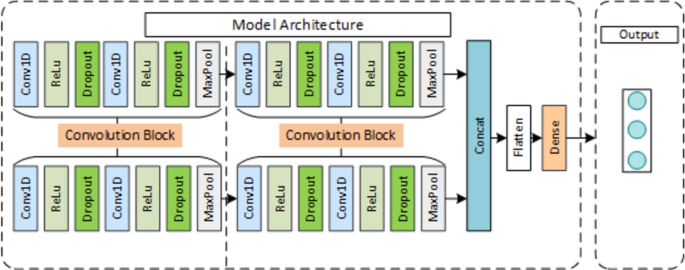
In this paper, a multi-channel feature fusion approach model shown in Fig. 5 was proposed as a comparison method to the MCDF model. The feature fusion model consists of two submodules to extract each sensor channel feature, a concatenation function to concatenate the features of each channel, a flattening layer to flatten the features, and a dense layer to build a fully connected layer. The submodel loads initial parameters from the 1D-CNN model pretrained on the UCI-HAR dataset and trains on our dataset. The categorical cross-entropy is used as the loss function. The submodule contains the same two sets of convolution blocks, as shown in Fig. 4.

Diagram of the multichannel 1D-CNN feature fusion (abbreviated as F–C) architecture for the HREA system.
To evaluate the overall performance of the model, the precision, recall and F1 score are used:
The precision is calculated for the model
$$\beginarraycPrecision\left(P\right)=\fracTP\left(TP+FP\right)\endarray$$
(13)
where TP is a true positive and FP is a false positive. The recall value is calculated as:
$$\beginarraycRecall\left(R\right)=\fracTP\left(TP+FN\right)\endarray$$
(14)
where FN is the false negative. The F1-Score is calculated as:
$$\beginarraycf1 Score\left(f1\right)=\frac2\times P\times R\left(P+R\right)\endarray$$
(15)
The weighted-avg value is calculated as:
$$\beginarraycweighted\; avg(P,R,f1)=\sum _n^i\fracN_iN_total*(P,R,f1)_i\endarray$$
(16)
where \((P,R,f1)_i\) is the Precision, Recall and \(f1 Score\) of the i-th class.\(N_i\) is the sample size of i-th class, \(N_total\) is the total sample size. The P, R, F1-score figures below all refer to the weighted average of P, R, F1-score, i is the ith sample classification and n is the total number of sample classifications.
link

