

For activity recognition, we employed a transformer encoder-based deep-learning model. An RGB camera captures the video frames and joint coordinates are extracted using Mediapipe open source framework. The extracted joint coordinates are further processed to identify the performed activity. Additionally, the captured coordinates are analyzed using auto-correlation and peak detection techniques to count the number of repetitions. Figure 1 presents an overview of the proposed framework. A detailed description of the proposed method is presented in the later sections.
Data collection
We enrolled multiple healthy participants for our study to perform different exercises. The demographic of participants is shown in the Table 1. All the participants signed the informed consent. The study was approved by the local Institute Ethical Committee (Humans) at Indian Institute of Technology Ropar file no. IITRPR/IEC/2023/025 dated \(1^{st}\) March, 2024 and all experiments were performed in accordance with relevant guidelines and regulations. Following the protocol, all participants were asked to perform different exercises to execute a certain number of repetition cycles. The protocol included 12 activities including rehabilitation exercises40. Table 2 presents the demographic of the performed activities. Among all, 11 activities (excluding idle) were used for repetition counting and the rest were all for training the transformer encoder-based deep learning model.
All the performed activities were recorded using a OnePlus 11R Android smartphone with a 50MP rear camera. Recorded videos were captured at a resolution of 720p at a frame rate of 30 FPS. The smartphone was mounted on a tripod at a distance of 2–3 meters from the participants. In total 96 videos were recorded, comprising 1480 repetitions.

Transformer model architecture for activity prediction.
Key points detection using mediapipe
Mediapipe framework has been used for predicting the body skeleton in the current study due to its reliability and good accuracy with low latency. Garg, et al. in their study have shown the results comparison of different deep learning models for Yoga pose estimation. In their study, it has been concluded that the use of mediapipe certainly enhances the performance of the system and is found to be quite effective for pose estimation41.
Mediapipe identifies 33 key landmarks on the human body. Each landmark is represented by the vector \([x_i, y_i, z_i, v_i]\) containing three spatial and one visibility factor. The visibility factor’s magnitude lies between 0 and 1, with zero corresponding to less visibility in case of occlusion or poor lighting and 1 for high visibility. After combining all landmarks, we get a feature vector of length D = 132 for each frame captured at a particular time instance: \(\textbf{a} = [x_0(f), y_0(f), z_0(f), v_0(f), \dots , y_{32}(f), z_{32}(f), v_{32}(f)] \in \mathbb {R}^{1 \times D }\), where the subscripts represent landmarks and f is the frame index or time-point. The output of MediaPipe Pose Landmark model is shown in Fig. 2.
Windows creation (data preparation)
We utilized sliding window mechanism to divide the entire sequence of frames into smaller segments (see Fig. 2). For the input frames sequence represented by a 2D matrix: \(\textbf{A}= [\textbf{a}_1, \textbf{a}_2, \dots , \textbf{a}_F]^{‘} \in \mathbb {R}^{F \times D}\), F is the number of frames in the entire sequence, and each \(\textbf{a}_f\) represents the joint-coordinate feature vector of a single frame with length D. The sliced data matrix can be obtained as:
$$\begin{aligned} \textbf{I}_m = A_{[m \times u]:[(m \times u) + N] } \in \mathbb {R}^{N \times D} \end{aligned}$$
(1)
Where, \(I_m\) is the \(m^{th}\) window matrix, u is the stride and N is the window size.
Deep learning model
In this study, we have utilized a transformer encoder-based architecture for activity identification. Figure 3 shows the architecture of the deep learning model. This architecture mainly consists of two parts: Firstly a transformer encoder and secondly the dense layers. The transformer encoder consists of multi-head self-attention and feed-forward layers. The vector \(I_m\) is given as an input to the transformer encoder.
The transformer model’s multi-head self-attention is an advanced technique intended to capture complex dependencies within a sequence42. Employing several parallel attention heads, improves on the conventional self-attention process. Each head uses its own set of query (Q), key (K), and value (V) matrices to carry out self-attention on its own. The self-attention mechanism uses the scaled dot-product formula to calculate the attention scores for a single attention head:
$$\begin{aligned} Attention(Q, K, V) = softmax \left(\frac{QK^T}{\sqrt{d_{model}} }\right)V \end{aligned}$$
(2)
where \(d_{model}\) is the keys’ dimensionality. By providing a probability distribution across the data, the softmax function makes sure that the attention ratings are normalized. In multi-head self-attention, learning projection matrices are used to linearly project the input embeddings into H distinct subspaces (heads): \(Q_h = X W^Q_h\), \(K_h = X W^K_h\), and \(V_h = X W^V_h\), where the projection matrices for the h-th head are \(W^Q_h\), \(W^K_h\), and \(W^V_h\). The following is how each head h calculates self-attention:
$$\begin{aligned} Head_h = Attention(Q W^Q_h, K W^K_h, V W^V_h) \end{aligned}$$
(3)
All heads’ outputs are concatenated and passed via a final linear projection:
$$\begin{aligned} MultiHead(Q, K, V) = Concat(Head_1, …, Head_H)W^O \end{aligned}$$
(4)
Where the output projection matrix is denoted by \(W^O\). The encoder layer incorporates a position-wise feed-forward neural network (FFN) after the multi-head self-attention. By adding non-linearity, this feed-forward network enables the model to further alter the representations. A residual connection and layer normalization come after both sub-layers (feed-forward neural network and multi-head self-attention).
The output of the transformer encoder is passed to the dense layers with the last layer followed by a Softmax layer outputting the activity predictions.
Activity repetition counting
For any motion to be considered periodic, a certain pattern must repeat itself after a particular interval of time. Each activity is unique and involves the movement of different body parts, which makes the repetitive counting tasks challenging.

This figure shows the body joint landmarks and the combined vector V with varying magnitudes of the participant performing an inline lunge activity. Here, \(f_0, f_1 \dots f_9\) are the frames at different time stamps.
Combined motion
To generalize the motion, we have combined the motion of all the joints by summing their velocity vectors \(\vec {v_m}\) for each frame (see Fig. 4). For our study, we included only x and y coordinates for velocity vector calculation. For matrix \(A’\) containing landmarks \(a’= [x_0, y_0, x_1, y_1, x_2, y_2, \dots , x_{32}, y_{32}]\) including x and y coordinates the velocity vector can be written as:
$$\begin{aligned} \vec {v’_m} = a’_m – a’_{m-1} \end{aligned}$$
(5)
Here, \(\vec {v’_m}\) is the velocity vector for frame m, \(a’_m\) is the landmark obtained for frame m and \(a’_{m-1}\) is the landmark vector for frame \(m-1\).
Data filtering
To compensate for the noises and disturbances which cause the magnitude of the vector \(\vec {v’_m}\) to be very high for an instant, the x and y components \(v’^x \text { and }v’^y\) are capped/limited to a certain threshold for both negative and positive values. This capping ensures a smooth operation.
$$\begin{aligned} v’^x= & \max \left( -\delta _{\text {limit}}, \min \left( v’^x, \delta _{\text {limit}}\right) \right) \end{aligned}$$
(6)
$$\begin{aligned} v’^y= & \max \left( -\delta _{\text {limit}}, \min \left( v’^y, \delta _{\text {limit}}\right) \right) \end{aligned}$$
(7)
Here \(\delta _{\text {limit}}\) is the capping threshold value. The combined vector V is the vector sum of all the velocity vectors of the body landmarks. The combined vector for the \(m^{th}\) frame is given as:
$$\begin{aligned} \vec {V’}_m = (\vec {v’}_m(0) + \vec {v’}_m(1) + \vec {v’}_m(2) + \vec {v’}_m(3) \dots \vec {v’}_m(j)),\hspace{0.2cm} j \in [0,32] \end{aligned}$$
(8)
Here, \(\vec {v’}_m(j)\) is the velocity vector of the \(j^{th}\) joint landmark for the \(m^{th}\) frame.
The capped values are further smoothened out using the exponential average. The exponential operation can be defined as:
$$\begin{aligned} V^x_m= & \alpha \cdot V’^x_m + (1 – \alpha ) \cdot V^x_{m-1} \end{aligned}$$
(9)
$$\begin{aligned} V^y_m= & \alpha \cdot V’^y_m + (1 – \alpha ) \cdot V^y_{m-1} \end{aligned}$$
(10)
Where \(V^x_m\) and \(V^y_m\) are the smoothed values of the x and y components of the combined vector \(\vec {V}_m\) respectively at the \(m^{th}\) frame. Also, \(V’^x_m\) and \(V’^y_m\) are the raw input values of the x and y components respectively at the \(m^{th}\) frame. And \(V^x_{m-1}\) and \(V^y_{m-1}\) are the previous smoothened value. The smoothing factor \(\alpha \in (0,1)\) determines the contribution of current vs historical values. Higher values of \(\alpha\) emphasize recent data. The \(\alpha\) value is dynamically adjusted via a deep learning model i.e. higher values for fast activities (run and jump) and lower values for slow activities.
This makes the system generalized for any kind of motion. The magnitude of this resultant vector \(\Vert \textbf{V}\Vert = \sqrt{(V^x)^2 + (V^y)^2}\) is later utilized for repetition counting using correlation.

This figure shows different axes: x, y, 45pos and 45neg. The combined vector \(V\) is shown in red. Here, x_proj, y_proj, 45pos_proj, and 45neg_proj are the projections along the x-axis, y-axis, 45-pos axis, and 45-neg axis respectively.

(a) Signed magnitude plot of the vector Z for the sit-to-stand activity. (b) Autocorrelation R plot of the vector Z. (c) Detected peaks in the autocorrelation vector R, indicating periodic repetitions in the motion.
Motion direction
The repetitive motion can be along any direction. For example, for squats, the motion is along the vertical axis. Whereas, for inline lunges, the dominating motion is along the diagonal axis. To get the directional information, we take the projections along the four axes: x-axis, y-axis, 45pos-axis and 45neg-axis (see Fig. 5). Here, 45pos axis is the axis \(+45^{\circ }\) to the x-axis and 45neg is \(-45^{\circ }\) to the x-axis. The unit vectors along the 45pos and 45neg axis are given as:
$$\begin{aligned} \hat{V}_{45pos}= & \left[ \frac{1}{\sqrt{2}}\hat{i} + \frac{1}{\sqrt{2}}\hat{j}\right] \end{aligned}$$
(11)
$$\begin{aligned} \hat{V}_{45neg}= & \left[ \frac{1}{\sqrt{2}}\hat{i} – \frac{1}{\sqrt{2}}\hat{j} \right] \end{aligned}$$
(12)
The projection is calculated for the velocity vector \(\vec {V}_m\) for a certain number of frames M. To get the major axis along which the motion is happening, we take the variance of the projections for M frames along the x-axis, y-axis, 45pos-axis and 45neg-axis. The axis with the highest variance value is considered the major axis. For the list of vectors \(U = [\vec {V}_0, \vec {V}_1, \vec {V}_2, \vec {V}_3, \dots \vec {V}_{m}]\) for \(m\in [0,M]\). The variance can be calculated as:
$$\begin{aligned} \text {Var}(U) = \frac{1}{M} \sum _{m=0}^{M-1} \left( \vec {V}_m \cdot \hat{a}_K – \mu \right) ^2 \quad \end{aligned}$$
(13)
Where, \(\mu = \frac{1}{M} \sum _{m=0}^{M-1} \left( \vec {V}_m \cdot \hat{a}_K \right)\) \(\vec {V}_m \cdot \hat{a}_K\) is the projection of the velocity vector \(\vec {V}_m\) onto a candidate axis \(\hat{a}_K\), \(\mu\) is the mean of the projections over \(M\) frames and \(\text {Var}(U)\) the variance of the projected values. Also,
$$\begin{aligned} \hat{a} \in \left\{ \hat{i},\ \hat{j},\ \frac{1}{\sqrt{2}}(\hat{i} + \hat{j}),\ \frac{1}{\sqrt{2}}(\hat{i} – \hat{j}) \right\} \end{aligned}$$
(14)
For x-axis, y-axis, 45pos-axis and 45neg-axis. The axis with the maximum variance is considered as the major axis. For the major axis K, the immediate projection value for the \(m^{th}\) frame is \(\vec {V}_m \cdot \hat{a}_K\). Here, \(\hat{a}_K\) is the unit vector along the major axis \(K \in [x, y, 45pos, 45neg]\).
Now, the projection \(\vec {V}_m \cdot \hat{a}_K\) can be negative or positive. For a positive projection value, the magnitude \(\Vert \textbf{V}\Vert\) is multiplied by +1, and for a negative projection value, it is multiplied by -1.
$$\begin{aligned} Z_m = \Vert \vec {V}_m\Vert \cdot \text {sign}(\vec {V}_m \cdot \hat{a}_K) \end{aligned}$$
(15)
Where \(Z_m\) is the signed magnitude (see Fig. 6) of the combined vector \(V_m\) for the \(m^{th}\) frame and \(\hat{a}_K\) is the unit direction along the major axis. Also,
$$\begin{aligned} \text {sign}(\vec {V}_m \cdot \hat{a}_K) = {\left\{ \begin{array}{ll} +1 & \text {if } \vec {V}_m \cdot \hat{a}_K \ge 0 \\ -1 & \text {if } \vec {V}_m \cdot \hat{a}_K < 0 \end{array}\right. } \end{aligned}$$
(16)
Autocorrelation
To identify repetitions, we utilized auto-correlation using Pearson correlation on the 1d vector \(Z = [Z_0, Z_1, Z_2, Z_3, \dots Z_q] \in \mathbb {R}^{1\times Q}\) for \(q \in [0, Q]\). The auto-correlation formula can written as:
$$\begin{aligned} \tilde{R}(\ell )= & \frac{\sum _{t=0}^{M-\ell -1} (Z_t – \bar{Z})(Z_{t+\ell } – \bar{Z})}{\sqrt{\sum _{t=0}^{M-\ell -1} (Z_t – \bar{Z})^2} \cdot \sqrt{\sum _{t=0}^{M-\ell -1} (Z_{t+\ell } – \bar{Z})^2}} \end{aligned}$$
(17)
$$\begin{aligned} R(\ell )= & \frac{\tilde{R}(\ell )}{\max \limits _{\ell } \tilde{R}(\ell )} \end{aligned}$$
(18)
Where, \(Z_t\) is the value of the signal at time \(t\), and \(\bar{Z}\) is the mean of the signal over all time steps. The lag \(\ell\) represents the shift in time ranging from \(0\) to \(Q – 1\), where \(Q\) is the total number of samples). The Pearson autocorrelation coefficient at lag \(\ell\), denoted as \(\tilde{R}(\ell )\), measures the linear correlation between the original signal and its shifted version by \(\ell\) steps. \(R(\ell )\) is the normalized autocorrelation, and \(\max \limits _{\ell } \tilde{R}(\ell )\) denotes the maximum value over all lags of the unnormalized autocorrelation. For this study, we set the value \(\ell = 1\).
Peak detection
Peak detection is performed to count the number of repetitions in the last M frames. For a 1d vector \(R=[R(0), R(1), R(2), \dots R(Q-l-1)]\), the peak detection is performed using \(find\_peaks\) function of the scipy.signal library. For peak detection, the height threshold was set to 0.7, prominence to \(0.8\times max(R)\), distance to 10 and width to 2 (see Fig. 6). The output of this function gives the frame indexes where the peaks were detected. For continuous peak detection and to limit the computational analysis, the size of the signed magnitude vector Z is limited by dropping the older values. The peak detection algorithm is explained in Algorithm 1.
Repetition counting algorithm (algorithm-1)
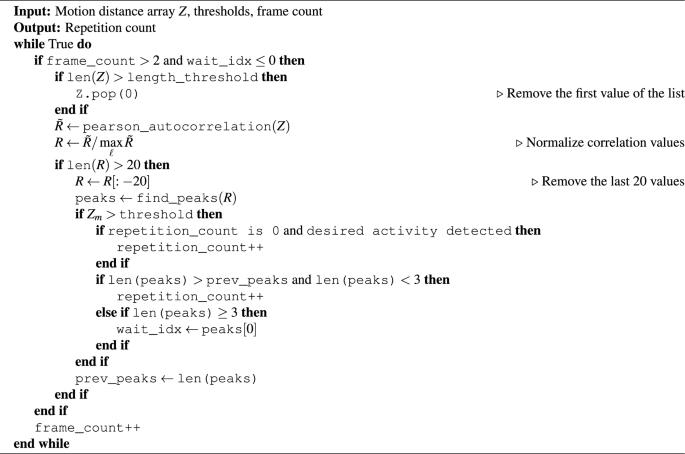
Autocorrelation-based repetition counting algorithm
The recurring patterns are detected by analyzing the autocorrelation time series produced from the signed magnitude vector Z. The key concept used is the temporal periodicity inherent in the repetitive actions and this appears as a regular pattern of peaks in the autocorrelation signal R (see Fig. 6). In this method, the velocity vector Z generated from the skeletal body joints coordinates, applicable thresholds and frame counts are taken as inputs. An iterative temporal development of motion data is analyzed.
Initially, the algorithm examines if a sufficient number of frames have been processed (\(frame\_count>2\)) and guarantees that the system is not currently in a waiting state (i.e., \(wait\_idx\le 0\)). If the length of the vector Z exceeds a predetermined threshold, the first data point is eliminated to keep a fixed-size window. The primary signal-processing step is to compute the Pearson autocorrelation of the current motion distance series. This autocorrelation signal \(\tilde{R}\) is normalized by its highest value to provide R, which improves numerical stability and ensures consistent peak analysis across varied magnitudes of motion.
To minimize the impact of trailing data and noise, the last 20 entries of R are trimmed. A peak-finding algorithm is then used to identify the resultant autocorrelation signal’s peaks. If the current maximum value \(Z_q\) exceeds a predetermined threshold (indicating a meaningful point), the algorithm compares the number of detected peaks to the prior observed count. The first repetition (for \(repetition\_count == 0\)) is detected and \(repetition\_count\) is incremented when the deep learning model identifies the user-specified activity. If the number of peaks has grown but is still less than 3, a repeat is assumed, and the repetition count is raised. If there are three or more peaks, the algorithm enters a waiting state and records the index of the first peak. This method prevents over-counting when there are quick or overlapping repeats.
Finally, the previous peak count is updated while the frame count is incremented. The loop runs continuously, allowing for continuous monitoring.
link