Figure 1 gives the overall components of our proposed ML-Driven rehabilitation approach for lower limb exercises. Unlike others in literature, our approach leverages a hybrid approach combining Convolutional Neural Networks (CNN), Fuzzy rule-based model, and K-Nearest Neighbors (K-NN) algorithms to provide a comprehensive solution for lower limb rehabilitation. We represent the details of each components in the following subsections.

The overall components of our proposed ML-Driven rehabilitation approach for lower limb exercises.
Due to the lack of publicly available video datasets of real stroke patient rehabilitation exercises, the research team collaborated with the Faculty of Medicine at King Chulalongkorn Memorial Hospital to record rehabilitation exercises performed by 30 experienced physical therapists in a clinical setting. Each therapist provided 5 videos demonstrating 3 different lower limb exercises from frontal and side views, which were deemed suitable for evaluating lower limb rehabilitation. The video data were created under the supervision of a rehabilitation doctor. The computational resources utilized in this study included an external camera and a computer with an AMD Ryzen 7 5800H processor, 16 GB of RAM, and an NVIDIA GeForce RTX 3050Ti GPU. Compared to the literature, this video dataset recorded in a clinical environment with experienced therapists is considered more reliable than others in literature for training the proposed ML-Driven rehabilitation model.
Lower limb recovery exercises
Our study aims to propose an ML based approach for lower limb rehabilitation in stroke patients. The research training is divided into two parts. Firstly, neurologist doctors provide exercise instructions and create 30 video datasets with various exercise types for post-stroke patients. Subsequently, the proposed model will be trained using this dataset, initially focusing on describing the human-centric aspects, such as pose, direction, and angle of movement of the patient, followed by the ML-Driven process in the second part of the training. Figure 2 gives the Fugl-Meyer Assessment (FMA) lower limb points39. The exercise evaluates the subject’s motor function related to the human brain. It includes testing the patellar, knee flexor, and achilles reflexes. The subject is instructed to flex the hip, knee, and ankle joints to their maximum range of motion while sitting in a chair, usually at the exact moment. Typically, both hip abduction and outward rotation occur simultaneously. To confirm the active flexion of the knee during this motion, the distal tendons of the knee flexor should be palpated. This research also emphasizes the FMA lower limb criteria.
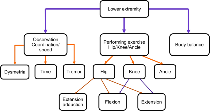
The Fugl-Meyer Assessment (FMA) assessment function of lower limb part for stroke rehabilitation5.
These hip, knee, and ankle point lower limb exercises target specific lower limb muscles and can help improve strength, coordination, and balance. The repetitive movements involved in these exercises can also stimulate the neural connections in the brain, helping to rewire and enhance the motor pathways damaged by the stroke. Regular exercise can also help to improve circulation and oxygenation to the brain, which can aid in the recovery process and support overall brain health.
Hip flexion
Patients with restricted mobility benefit significantly from this leg exercise since they can use their arms to support their legs. To start this exercise, use the patient’s hands to lift their affected leg into the chest. Hold there for a second before slowly letting the leg back down. Repeat on the other leg. This type of exercise targets the hip flexor muscles and helps to improve their strength and flexibility. These muscles can aid in walking and rising from a chair. These exercise positions are illustrated in Fig. 3.

From left to right sub-figures: Example hip flexion exercise on left leg.
Hip external rotation
Compared to the first exercise, hip external rotation is more complex but still suitable for patients with limited mobility. To facilitate movement, start by putting a towel beneath the troubled foot. Then, use the subject hands to assist the affected leg and slide the foot toward the mid-line. Then, push the patient’s leg outwards, using hands for assistance if it is essential. This type of exercise targets the muscles that rotate the hip outward, which can help improve mobility and stability in this joint. This can be particularly important for post-stroke patients who experience difficulty with weight-bearing activities due to hip weakness. These exercise positions are illustrated in Fig. 4.

From left to right sub-figures: Example hip external rotation exercise on right leg.
Knee extension
For stroke patients, a more challenging leg exercise is knee extension. To begin, it necessitates considerable leg movement. It is starting the exercise while seated. Next, straighten the left knee and stretch the leg parallel to the ground. Instead of locking out the knee, try to keep it supple. After that, slowly lower the foot to the ground. After that, repeat with the right leg, switching between the right and left legs. This type of exercise focuses on strengthening the muscles that control knee extension, which can help to improve walking speed and stability. These exercise positions are illustrated in Fig. 5.

From left to right sub-figures: Example knee extension exercise on right leg.
Table 1 describes the three exercises and how to perform them. This research aims to create an ML-based model for aiding in the clinical diagnosis and home rehabilitation of post-stroke patients. We checked our model in both home and clinical or hospital-based environments.
MediaPipe pose
MediaPipe Pose is an ML solution for high-fidelity body pose tracking, inferring 33 3D landmarks and background segmentation masks on the whole body from RGB video frames utilizing Blaze Pose research that also powers the ML Kit Pose Detection API. Current state-of-the-art approaches rely primarily on powerful desktop environments for inference. In contrast, the proposed method achieves real-time performance on most modern mobile phones, desktops/laptops, python, and the web. The MediaPipe Blaze Pose model is based on the COCO topology, consisting of 33 landmarks across the torso, arms, legs, and face, as presented in Fig. 6. However, the COCO key points only localize to the ankle and wrist points, lacking scale and orientation information for hands and feet, which is vital for practical applications like fitness and dance. Including more key points is crucial for the subsequent application of domain-specific pose estimation models, like those for hands, faces, or feet. With BlazePose, the authors present a new topology of 33 human body key points, a superset of COCO, BlazeFace, and BlazePalm topologies. This allows them to determine body semantics from pose prediction alone, consistent with face and hand models.
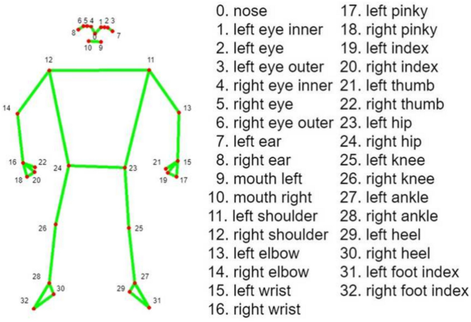
Demonstration of 33 landmarks detected on the human body using MediaPipe40.
For pose estimation, the two-step detector-tracker ML pipeline is utilized. This pipeline first locates the pose region of interest (ROI) within the frame. The tracker subsequently predicts all 33 pose key points from this ROI. Notably, the detector is run only on the first frame for video use cases. The pose estimation component of the pipeline predicts the location of all 33 key points with three degrees of freedom each (x, y location, and visibility) plus the two virtual alignment key points described above. The model uses a regression approach supervised by a combined heat map/offset prediction of all key points41. Specifically, during training, the pipeline first employs a heatmap and offsets the loss to train the center and left tower of the network. It then removes the heatmap output and trains the regression encoder, thus effectively using the heatmap to supervise a lightweight embedding.
It is important to note that exercises should be tailored to each individual’s specific needs and abilities. Therefore, it is crucial to stress that these exercises should be performed under the guidance of a physical therapist. Moreover, the therapist will be able to oversee the patient’s progress and modify the treatment plan as necessary.
Training of proposed models
In this research, we implemented two separate machine learning models: one is K-NN, and the other is the hybrid rule-based model. In the hybrid model, the CNN model draws the human skeleton and shows the joint points. Fuzzy logic rules are applied to extract the specific joint angle and count the exercise of the hybrid model. The k-NN model visualizes the exercise graph based on the train data set and counts the perfect exercise. A predefined machine learning model is used for skeleton detection and is an input in both cases.
From the video or real-time human skeleton pose tracking system, a general framework is shown in Fig. 7. MediaPipe ML algorithm tracks the pose landmarks in this way. The skeleton’s media pipe draw depends on the input RGB image and generates the heatmaps of the key point locations. The work of crucial point visibility can be described in this way: the input frame detects pose alignment with heatmaps, and pose landmarks detect pose alignment. The network architecture of the regression with heatmap supervision is shown in Fig. 8. The 8-by-8 frame size to 64-by-64 frame size image is interconnected with heatmap input RGB and key point visibility.
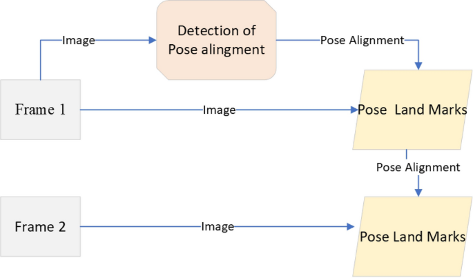
Model Input frame to pose landmarks.
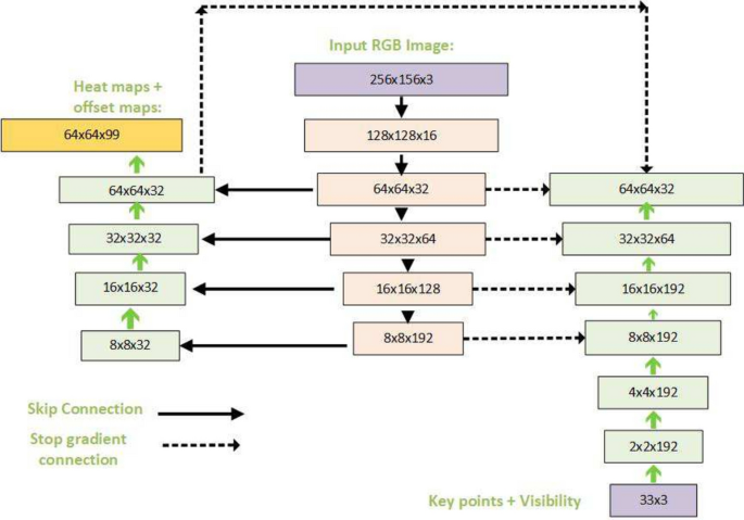
Tracking network architecture: regression with heatmap supervision.
The machine learning-based model output is accuracy, and it visualizes the graph of accuracy that it learns from the accurate video dataset created for this research study. For training purposes, the dataset was used from King Chulalongkorn Memorial Hospital, consisting of 30 subjects performing post-rehabilitation exercises, all confirmed by a neurologist and a physiotherapist. Here, the data is used to train and evaluate the K-NN algorithm through the training process. Then, the angle of every video data is extracted. Later, it adjusted with the extracting angle and FMA logic. The hybrid noble model for the automatic angle measurement of the exercise in the desired point moving part according to the FMA method, or we can set our own defined rule for the patient, which was not previously done using any ML model. We employed MediaPipe to draw the human skeleton over the patient’s body. We chose the Blaze Pose Lite MediaPipe, which has a 33 key point topology, for its updated version and the additional information it provides, including the number of joints and critical points, which aids in diagnosing the patient. This model can measure any specific joint angle from 33 joint points and gives the status of the angle’s changing while counting the reps. Our approach enables doctors to monitor their patients’ progress efficiently without needing a stopwatch or assistance counting and tracking the rehabilitation exercises. Furthermore, with scale and rotation, additional information, such as hands, faces, and feet, helps diagnose.
Fuzzy rule-based model
The summary of the proposed fuzzy rule-based hybrid ML model is described in this section. The proposed model learns the human body’s skeleton position, which are visualized in Figs. 9 and 10. With the movement of the body, the skeleton will also move. It will also track how many exercises have been completed and display that information on the screen. The machine learning part of this, which we already discussed above, is that the heat map generation from the image frame and pose alignment draws the body’s skeleton. Moreover, counting the exercises performed is also very important because these are compared with the medicine dose. Both of these things are addressed in the hybrid model. Detecting the whole-body skeleton in this coding screenshot uses MediaPipe computer graphics. The first step is to call the media pipe pose and change the screen image to RGB. Then, detection is made, and the detection is drawn. The user can press a key to stop the process. The human body skeleton’s key points, or joint structures, are extracted using MediaPipe computer graphics, and 33 key points are identified. The landmarks are used to identify the 33 key point joints and the key points are determined based on the researchers’ requirements. A hybrid model architecture is used for the post-rehabilitation phase. The data is one for machine learning pose estimation and the other for proper angle representation.
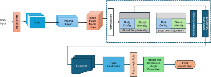
Proposed model framework for human pose refinement and angle calculation process.
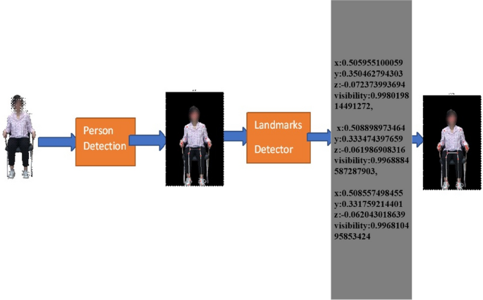
Human person drawing the MediaPipe landmark and extracting the landmarks point.
The 2D system has a two-point X axis, described from left to right, and the Y axis is the point from bottom to top. For this model to calculate the joint angle movement, we must measure the 3D skeleton point. The 3D space point is used to measure the point of the media pipe skeleton. X, Y, and Z, and after that, it will be visible. We can also call it visualization or detecting skeleton points. Figure 10 shows the example detection of the human skeleton from the human body through the proposed method and how it extracts the landmark points of body joints.
$$\begin{aligned} ax+by+cz+d=0 \end{aligned}$$
(1)
Here, we give our lower limb part 3D value with visibility. Later, we reduced our 3D points to 2D points. In Eq. (1), we have the x, y, and z for every joint point. x, y, and z represent the positions of the point along the x-axis, y-axis, and z-axis. These three points represent the 3D visualization of each floating-point joint point. Visibility is the confidence level in showing the point on the screen. It is determined by 0 and 1; above 0.9, it has high confidence in visibility. Equation (1) represents the plane of 3D space, where a, b, and c are the coefficients of x, y, and z, and d is a constant that determines the plane’s position. It also represents the distance from the origin.For 3D joints, our model output and visibility are as follows.
$$\begin{aligned} \text {Left Hip:} {\left\{ \begin{array}{ll}x = 0.5340\\ y = 0.4754\\ z = -0.0036\\ visibility = 0.9999\end{array}\right. } \\ \text {Left Knee:} {\left\{ \begin{array}{ll}x=0.5408\\ y=0.5138\\ z=-0.1875\\ visibility=0.9978\end{array}\right. } \\ \text {Left Ankle:} {\left\{ \begin{array}{ll}x=0.5396\\ y=0.7088\\ z=-0.1298\\ visibility=0.9969\end{array}\right. } \end{aligned}$$
The above shows the value of x, y, and z for the particular landmark points of the left hip, left knee, and left ankle. 3D key point representation of the hip, knee, and ankle are the most important parts of our lower limb exercise. The 3D representation of key points in the representation is mathematically shown above for the left hip, left knee, and left ankle in their 3D positions.
We need to calculate the angle for the most important part of the rule-based model. To calculate the angle, we must set the rules. When we define the rules in Python and set the rules for determining the joint angle when we perform the exercise, we need the three-point starting point, mid-point, and end point. When the starting and ending points of the mid-point are changed, the degree of angle of the mid-point changes accordingly. The mathematical rule set for angle also describes the rules for radian and angle. We convert the 3D point into a 2D point for ease of calculation. The joint angle was calculated as the difference in angle between two adjacent segments’ longitudinal axes. These segments comprise three points in the 2D space: the beginning, the center, and the end. The neighboring segments for the knee joint angle were the lower limb and the crus, respectively, from knee to ankle. The measurements made for the knee and hip joints in this investigation.
Figure 9 shows the proposed method framework for identifying human landmarks. In this case, the model’s input is the RGB frame, which is resized with the convolutional and pooling layers. The base network predicts the pose with 33 landmark points.

Flowchart of proposed fuzzy rule-based model for lower limb rehabilitation.
$$\begin{aligned} \left[ \begin{array}{l} X_{C K 1} \\ Y_{C K 1} \\ Z_{C K 1} \end{array}\right] =R\left[ \begin{array}{l} X_{K 1} \\ Y_{K 1} \\ Z_{K 1} \end{array}\right] +T \end{aligned}$$
(2)
$$\begin{aligned} \bigg \lceil u=\left( \frac{x}{z}\right) * f_x+c_x v=\left( \frac{y}{z}\right) * f_y+c_y\bigg \rceil \end{aligned}$$
(3)
In Fig. 11, the blue arrow indicates the step-by-step in the flowchart. The blue arrow indicates the yes condition, and the black arrow indicates the no logic condition. In Equation (2), the model working is derived using mathematical rules to extract the joint representation angle.
In Eq. (2), K1 coordinate system
$$\begin{aligned} \left[ \begin{array}{l} X_{C K 1} \\ Y_{C K 1} \\ Z_{C K 1} \end{array}\right] \end{aligned}$$
the coordinates all refer to the same place in the coordinate CK1 system. The 3×3 rotation matrix R describes the orientation of the CK1 coordinate system with the K1 coordinate system. The unit vectors of the CK1 coordinate system expressed in the K1 coordinate system are shown in the columns of R. All refer to the same place in the CK1 coordinate system. The orientation of the CK1 coordinate system in relation to the K1 coordinate system is described by the 3×3 rotation matrix R. The unit vectors of the CK1 coordinate system expressed in the K1 coordinate system are shown in the columns of R.
The position of the CK1 coordinate system with the K1 coordinate system is indicated by the translation vector \([T_x,T_y,T_z]\).
It reflects the displacement in the \(K_1\) coordinate system from the origin of \(K_1\) to the origin of \(CK_1\). Equation (3) represents the values of \(u\) and \(v\), denoting the point’s horizontal and vertical coordinates in the picture plane. The camera’s focal lengths along the horizontal and vertical axes are \(f_x\) and \(f_y\) respectively. In terms of pixels, it indicates the separation between the image plane and the camera’s center.
The intersection of the camera’s optical axis and the picture plane is the primary point of the camera, and its coordinates are \((c_x, c_y)\).
The vector in pixel coordinates \(\textbf{u}=[u_x,u_y]\) denotes the direction from the camera’s center to the projected 3D point in the image plane. It represents the angle calculation derived through the vector. The vector denoted by \(\textbf{v} = [v_{x}, v_y]\) points from the camera’s center to an image-plane reference point, such as the main or image’s center.
The symbol \(\cdot\) denotes the dot product. \(|\textbf{u}|\) and \(|\textbf{v}|\) represent the magnitudes of the two vectors. The result of multiplying the lengths of the two vectors by the cosine of the angle that separates them \(\theta\) is denoted as \(\mathbf {u \cdot v} = |\textbf{u}| \cdot |\textbf{v}| \cdot \cos {\theta }\).
Machine learning representation
The appropriate samples should be collected for the training set to build a good classifier for each terminal state of each exercise (e.g., “up” and “down” positions for rehabilitation exercise). Collected samples must cover camera angles, environmental conditions, body shapes, and exercise variations. This work creates the training video datasets by following the lower limb exercises. The stroke recovery exercises focus on the legs to help affected patients improve or enhance their gait (way of walking) and balance. This type of training of the legs can also help reduce the risk of falling, which is a priority for all stroke survivors. This type of exercise is also very effective for elderly people. The hip flexion, external hip rotation, and knee extension exercises are described and presented in Figs. 3, 4 and 5.
Figure 12 shows the hip flexion exercise step by step from (a) to (e). The overall stroke rehabilitation monitoring processes are evaluated, as shown in Fig. 13, based on the MediaPipe Pose model from Google AI. Google Colab loads the MediaPipe Pose model into the Keras platform to support training ML models. All the training image datasets are uploaded to Google Drive to accelerate the training pipeline and applied to the 33 human body key points. Next, the key-pointed images are loaded to the K-nearest neighbors (K-NN) algorithm to classify the rehabilitation activities. Then, the trained ML model is implemented as the backend engine for the web apps of the stroke system via the platform to build webapps or even mobile applications. The mathematical equation of k-NN is given in Eqs. (4) and (5).

Training process angle calculation among HIP, KNEE, and ANKLE points. (a) sitting in the normal pose (b) start moving of left leg (c) target position (d) start moving the right leg (e) right leg targeted position.
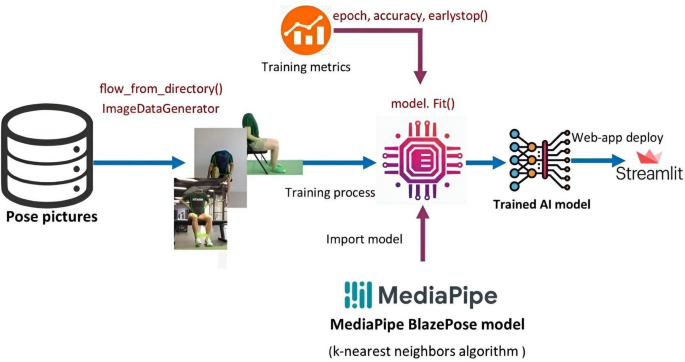
The overall pipeline process of training K-NN machine learning model.
$$\begin{aligned} \begin{array}{r} d\left( x, x^{\prime }\right) =\sqrt{\left( x_1-x_1^{\prime }\right) ^2+\cdots +\left( x_n-x_n^{\prime }\right) ^2} \\ \end{array} \end{aligned}$$
(4)
$$\begin{aligned} \begin{array}{r} P(y = \mid j \mid \mid X=x)=\frac{1}{K} \sum _{i \in A} I\left( \left( y^{(i)}=j\right) \right. \end{array} \end{aligned}$$
(5)
Equation (4) represents the Euclidean distance between two n-dimensional points, x and \(x’\). Now \(x = (x_1, x_2, \ldots , x_n)\) represents an n-dimensional point with n components, while \(x’=(x_1′,\ldots ,x_n’)\) represents another n-dimensional point with n components. The expression \((x_i – x_i’)\) represents the difference between the i-th component x and the i-th component of \(x’\). The expression \((x_i – x_i’)^2\) represents the square of the difference between the i-th component of x and the i-th component of \(x’\).
Equation (5) represents the conditional probability of a discrete random variable y taking the value j, given that another random variable X takes the value \(\kappa\). In this equation, \(P(y=|j||X= x)\) represents the conditional probability of \(y=|j|\) given \(X=x\). K is a normalizing constant that ensures that the probabilities sum up to 1. \(\sum _{i\in A}\) represents the sum over all i in set A, a subset of the index set of the data points. \(I((\hat{y}^{(i)}=j))\) is an indicator function that evaluates to 1 if the i-th data point has the label \(\hat{y}^{(i)}=j\), and 0 otherwise.
The K-NN model training pipeline process is done via the Google Colab environment. The model’s accuracy values are shown in Table 2 in the experimental results section. The accuracy is calculated as the total number of recognized exercises by the trained K-NN model over the total number of exercises done. More datasets of those exercises can be collected to retrain the model to improve the accuracy performances.
Vector format of angle extraction
Equation (6) gives the vector format of angle extraction. The \(\varvec{a}\) and \(\varvec{b}\) represent two neighboring segments with vectors \(\varvec{a}\) and \(\varvec{b}\), where the angle between \(\varvec{a}\) and \(\varvec{b}\) is equal to \(\varvec{\theta }\). The dot product is defined as the product of the vectors’ magnitudes multiplied by the cosine of the angle between them.
$$\begin{aligned} \begin{aligned}&{\varvec{a} \cdot \varvec{b} } =|\varvec{a}||\varvec{b}| \cos (\theta ) \\&\cos (\theta )=(\varvec{a} \cdot \varvec{b}) /|\varvec{a}||\varvec{b}| \\&\varvec{\theta }=\arccos \frac{\varvec{a} \cdot \varvec{b}}{|\varvec{a}||\varvec{b}|} \\ \end{aligned} \end{aligned}$$
(6)
Geometry format of angle extraction
We used geometric calculation to determine how accurate the angle prediction is, based on the hybrid fuzzy rule-based ML model. We later validated this angle with the mathematical calculation of the visualization angle. Here, the desired angle is cos A, which is from Euclidean geometry. Through Euclidean geometry, it is possible to figure out the angle joint between two rays. In this case, it is assumed that one ray is AB, and another is AC, and the distance BC determines the degree of the angle formed by the two rays. We can define AB = c, AC = b, and BC = a. The geometric equation is given below.
$$\begin{aligned} \begin{aligned}&\cos (A) = \frac{ b^2 + c^2 -a^2 }{2bc} \end{aligned} \end{aligned}$$
(7)
Equation (7) describes the relationship between the cosine of an angle \(A\) (equivalent to \(\theta\) in a triangle) and the lengths of its sides. In this equation, a, b, and c are the lengths of the sides of the triangle. A is the angle opposite to the side of length a. cos(A) is the cosine of angle A.
Statistical analysis
We measured knee and hip joint angles at the starting and end range of the exercise using our hybrid rule-based model. A total of 30 physical therapists performed hip flexion, knee extension, and hip external rotation with 10 repetitions separately for each leg. The mean range of motion was \(40.20^\circ\) degrees, with a median of \(40^\circ\) degrees and a standard deviation of \(16.721^\circ\) degrees, calculated for each joint with \(95\%\) confidence intervals. To assess the reliability of the measurements, we analyzed variance (ANOVA) using a linear mixed effects model in Python. The model was fitted with the formula range of motion group’. The resulting intraclass correlation coefficient (ICC) was 0.99, indicating perfect group agreement. Additionally, using G*Power (Version 3.1), a statistical power analyses, we calculated the sample size needed to detect a significance level of 0.05 or less with a power of 0.96 based on the correlation coefficient of the range of motion. The calculated sample size was 600. Assuming 10 independent trials per exercise for each leg, 30 subjects were required. Statistical analysis was performed using Python.
link
